In this page I aim to outline my process for selecting, downloading and processing point cloud LiDAR data into a mesh, to be used for sound level prediction in L-Acoustics Soundvision.
This page is a work in progress, so there’s probably a lot of errors and omissions – please let me know of any comments you may have via the contact page.
Where I’ve made estimations that effect the accuracy of the model, I’ve tried to highlight them in Red and subsequently explain why I deem them acceptable. I’m not a surveyor, so I’m happy to be proved wrong on any of these points.
Finally, please remember that these plots are not going to be 100% accurate, and a small error in this process could give you entirely the wrong data. Trust, but Verify with your own measurements.
Step 1: Finding your site in google maps
So to begin with we need to know where the site is geographically, so that we can make sure that we’ve got the mesh correctly aligned to give us the most accurate terrain data. Generally at this point I don’t have access to a detailed site map, so providing there’s been no changes to the site the easiest way is to find the site on google maps, switch to satellite images, and locate the stage in question using some detective work and last year’s public site map.
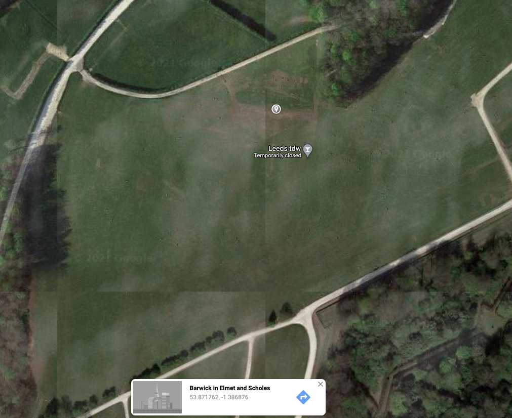
The image above is (I think) the main arena area for the Leeds Festival Main Stage, and an outline can be seen in the grass quite clearly where the stage sat. This gives us two bits of information:
Firstly the rough GPS position of the downstage edge centre can be found by clicking on the map and reading the numbers at the bottom (53.871762N 1.386876W)
Although this is almost certainly not centimeter accurate, I’m making the assumption that it’ll be within a ballpark of plus or minus 1m of the exact position, and this can always be revised with a more accurate position later on if one can be found.
Secondly we can get a rough compass bearing for the angle that the stage is sat at, which I estimated to be 185.5 degrees south.
Also a wild estimation by a very rudimentary method of sticking a post-it to the screen and then drawing a line in Autocad, however so long as it’s within a couple of degrees and the site isn’t crazy we should be onto a winner.
If we do have a site map at this point, it might be worth selecting a point that’s easier to identify, such as a crossroads or junction, and using that as our reference. Additionally if you have access to survey grade GPS kit (with GNSS/RTK capabilities), these points could come from a local measurement on site.
It’s important to note the coordinate systems used in each of these places – google maps uses a fairly standard system called WGS84, which is the same one that’s used for GPS systems. There are some issues with using this in the UK, such as its height isn’t constant across the country from east to west, and that the entire co-ordinate system is slipping across the land about 2.5cm per year in a north easterly direction. These issues are important to land surveyors, but given that we’re rarely considering an area wider than 500m or so and the absolute height is not important to us, we should be okay using these without much problem.
The North direction that Google maps uses is grid north, so it might be worth noting that it won’t exactly line up with magnetic north if you’re using a compass to verify a plot on site.
Step 2: Finding the Grid reference of the stage
For step 3, we’ll need both an OSGB 2 figure grid reference, and the absolute coordinates of our centre stage point relative to the OSGB Datum so that we can locate and place our stage within the arena. These grid references are specified as a “Northing” and “Easting” (rather than latitude and longitude) and represent the absolute number of meters north and east of the specified reference point or “datum”.
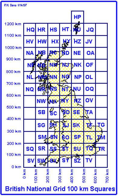
Looking at the image on the left, we can see that each 100km grid square in the British national Grid is given a 2-letter code, and this is the code that you see at the start of the grid reference, the numbers that follow will define a smaller square inside, 10km x 10km if it’s 2 numbers, 1km x1km for 4, 100m x 100m for 6…
So we need to convert our WGS 84 Lat/long to an OSGB36 co-ordinate, which can be done manually if you really like maths, but I’ve been using this website:
Inputting the Lat/long from step one in the format I wrote it in (53.871762N 1.386876W ) returns the OSGB36 grid reference:
OSGB36 Grid ref: SE 4041241902
10 digits, 5 for each direction, so this represents a 1m square on the map
Which from our geography lessons we’ll recognise (maybe) as a 10 figure grid reference, so the 1st and 6th digits can be taken to get our 2-figure reference:
2 figure Grid Ref: SE44
This represents a 10KM square on the map.
And then if we copy and paste the 10-figure grid reference into the search box again, it’ll give us some more information, including a row of text boxes where the first one says something along the lines of:
X=440412&Y=441902
These values are important as they represent the absolute number of meters that we are North and East of the OSGB36 datum, which is off the end of the Scilly isles in the South west corner of the British Mainland – but more importantly this is also the datum used in the LiDAR Data.
Step 3: Finding and Downloading the LiDAR data
Now this is the point where it could all fall apart, as there’s not LiDAR data for the whole country, so some locations need another method. (I’m looking at you Dorset) But thankfully I checked this one so we’re good. Coverage can be checked here:
But assuming you do have coverage for your chosen area, we now need to go to the correct website to download the data:
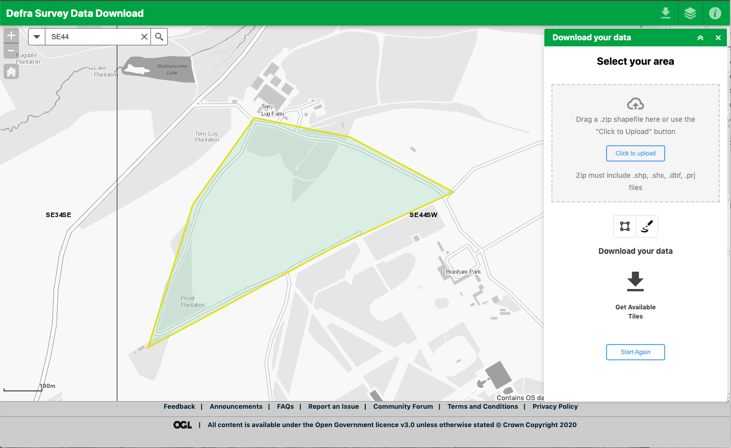
Once on this page you need to click “Show more” under ”Data Links” and then select “Survey data”. This will take you to a map interface, and if you enter the 2 figure grid reference from above (SE44) in to the search box and hit enter, you’ll end up looking at the right place. The first thing you’ll notice is that there are 4 grid squares for SE44 – SE44NE, SE44NW, SE44SE, and SE44SW – these split the 10km grid squares into 4x 5km squares to make the laser data more manageable. We’re looking at SE44SW in this case.
Zoom in and find the same area that you’ve got in google maps, and then used the download data symbol in the top-right to open the “Download your data” menu. Now you can use the lasso tool to draw a rough line around your chosen area, double-clicking the last point to close it off:
Once you’ve got your area selected, click the “Get available tiles” link in the download panel. Here we’re looking for the “Point Cloud” Data – there’s usually a couple of options here and I’d suggest downloading every point cloud set they’ve got, as it’ll offer you any set that has points within the SE44SW tile, and not all of them will necessarily cover the festival site. They’ll download as zipped folders and inside will be a selection of .laz files.
Step 4: Processing in CloudCompare
I found a free bit of software called CloudCompare (https://www.danielgm.net/cc/) that is built for manipulating point clouds, it runs on Win/Mac/Linux so should be fairly accessible for anyone who wants to do this. But before we jump into this, first I’m going to get a bit nerdy with what a point cloud is and what we’re doing with it.
What’s a Point Cloud?
A point cloud is generated by a scanning laser and can be used to generate a very accurate map of the 3d environment it’s scanning. The laser scans back and forth, pulsing a laser and watching for the returns as it bounces off objects
For each pulse of the laser it records a number of return times and intensities, for example if it hits the edge of a leaf but then also hits the ground below, you’ll get two “returns” from the same pulse. All of these returns are recorded as a point in 3d space, and before long you’ve got thousands of points arranged in a “cloud”.
We need to make a surface out of these points, which we can do by linking all of the dots together to create a “Mesh” of triangular surfaces, but to start off with there’s going to be far too many points and we’ll end up with too many surfaces for Soundvision to handle. So we need to do some filtering and subsampling of the points to get down to a manageable amount before we create our final Mesh.
Importing into CloudCompare.
Once you’ve got CC (CloudCompare) installed, find your .laz files in finder, select them all and drag them onto the main screen area of CC. It’ll start importing the files and pop up with this message box:
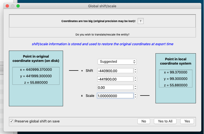
The Laser points are specified in absolute meters from OSGB36 Datum, so it’s telling us that all the points are 400km north and east of the origin, and that it’d like to move them closer to help with its processing. If we tick the “Preserve global shift on save” box, then the values here don’t really matter, so make sure the box is ticked, click “yes to all” and then it’ll start importing the data.
Trimming data down to the required area.
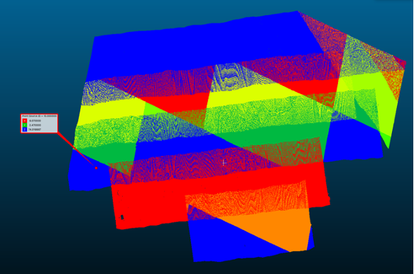
Once all the data is imported, you’ll get some great multi-coloured patchwork of points that don’t seem to tell you a whole lot. By selecting the point picking tool (top left toolbar, looks like a silver pointer and target) you can locate where your datum is by trial and error, which will give you an idea of the area you’re looking to process. Remember that at this point you could have up to 25 sq Km of data, and realistically we need 1% of that for a 500m x500m arena.
So we can start by getting rid of all the points we don’t need, so let’s set the view mode to “top” (Left hand tool bar, wireframe cube with orange top), select all of the laser files in the top left pane, and then select the Segment tool (Top toolbar, scissors). This will bring up a smaller toolbar in the top right corner that allows you to turn on rectangular selection, and then select a portion of the points. I’d suggest going wide at this point as it’s easier to delete parts of the mesh that you don’t need than going back to re-create a larger mesh.
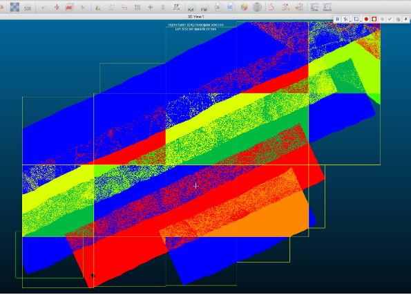
Pressing the “segment in” (polygon filled in with orange) button will show you a preview of the selected area with the other points removed, then you can click the “Confirm and delete hidden points” button to get rid of everything you don’t need. You should then end up with one or two point clouds and a load of empty folders in the DB tree. You can delete all the empty folders, and then you can merge the remaining point clouds into a single cloud using the merge tool in the top left toolbar.
Processing
Now that we have a single point cloud for our chosen area, we need to start processing it to make a mesh, so let’s rename the point cloud something sensible like “input cloud”.
Next we’re going to use the Rasterise tool to create a mesh out of all of the points, so first click the checkerboard icon on the top toolbar and this box will appear:
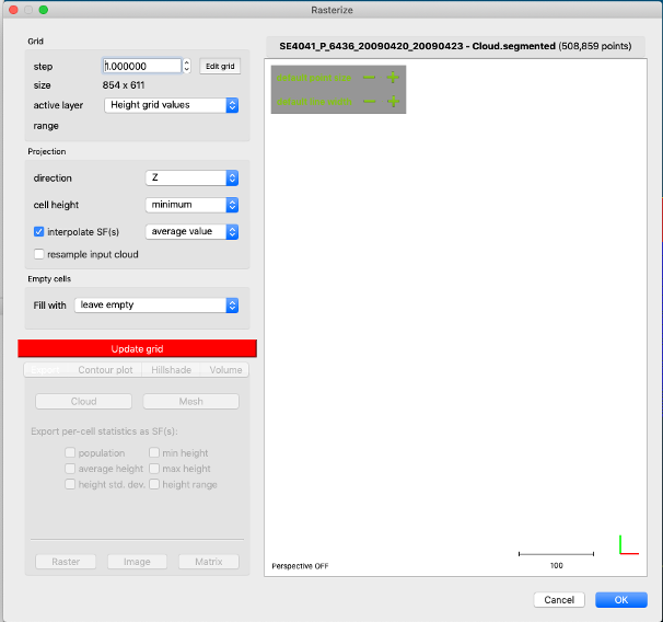
We need to make sure that the Cell height is set to “minimum” as this will pick the last laser return (which should hopefully be the ground, not a leaf/cable) and then hit the big red “update grid” button. Once that’s done you’ll get a pretty picture on the right hand side, then you can press the “Mesh” button and then “OK”
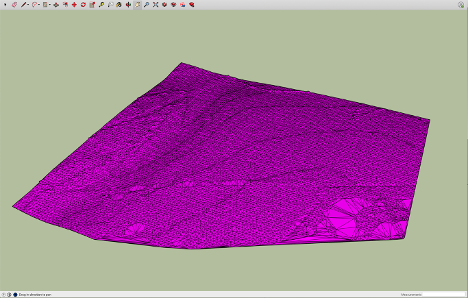
There will now be an “input cloud.mesh” item in the db tree, and within it there will be a “vertices” item. If we orbit this mesh and look across it we will probably see lots of spikes where trees have caused the mesh to pull up to include these points, and obviously we don’t want that in our plot.
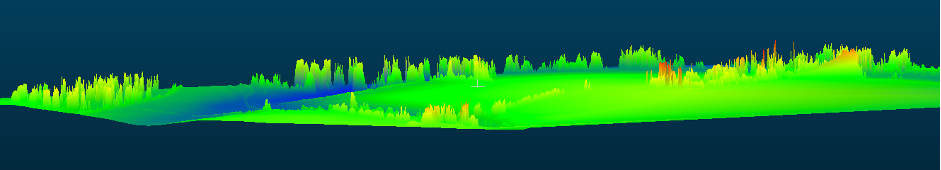
So this is possibly the most complex part of the processing – we need to get rid of points above the ground but leave the points that are actually at ground level. One way we could attempt this is to use a “Statistical Outlier Removal” tool, which considers each point and a specified number of points around it, and will remove it if it falls far enough outside of the whole range of heights. This works for cleaning individual trees out, but around heavily wooded areas the average height is still going to be significantly far away from the ground that we’ll get some “mounds” appearing where they don’t exist.
Thankfully some boffins have come up with a slightly more reliable way of filtering points called a “Cloth Simulation Filter”. This is designed to follow the terrain and trim away any trees/bushes so is pretty much perfect for what we want. You can start it by clicking the CSF symbol in the RHS toolbar.
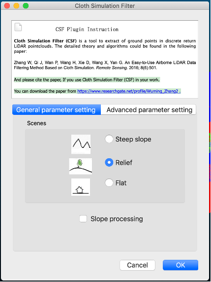
Just use the default options and press OK - This returns a lot cleaner set of points, and you can see where it’s removed lots of points in the wooded areas:
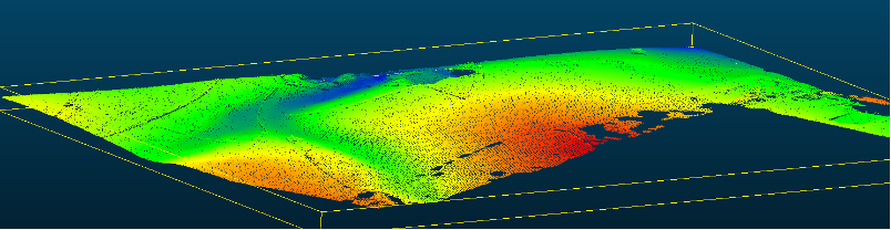
At this point I can see the field boundaries a lot more clearly so I’m going to use this opportunity to segment the cloud again, to get rid of some of the area I know I won’t need.
Once this is done we need to reduce the number of points in the cloud by using one of the subsampling methods available to us:
Random reduces the number of points to the specified number, which is helpful, but the size of the tiles in your mesh will be heavily dependent on the area you’re covering, so it’s not ideal for us.
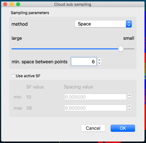
Space allows you to define a minimum separation between points, 6m for example, and then deletes all the rest of the points, resulting in a random mesh covering the full area, with all the tiles being roughly the same size.
Octree gets rid of a certain number of points dependent on a specified level, leaving you with a neat, square grid – however the final number of points is based on how many points there are to begin with, so the output mesh can vary drastically in size depending on how many points there were to begin with.
So select the vertices.clean(.segmented) and open the subsampling tool (top toolbar, red/blue points) and choose your “Space” and set it to 6m.
Finally, we can use the raster tool to create another mesh in the same way that we did above, then select this mesh in the DB tree and go to File>Save… and select DXF geometry as the file type.
Step 5: Importing and Aligning in Sketchup
Now we can import our mesh into sketchup, trim it down further and add any site features from the site map that might be helpful like the stage, FOH tower, delay positions… If you start with one of the template files, make sure that you delete the person from the origin before you start.
When importing DXFs to sketchup it’s important to go into the import settings and make sure that the units are set correctly, in this case they should be set to meters. The mesh will import miles from the axes so we need to find it first using the “Camera>Zoom Extents” function.
Once we’ve got it we need to shift it back to the origin, so select the mesh, select the move tool (M), click a point on the mesh to start moving it, making sure to press the right arrow to lock movement to the X (red) axis. Slide it towards the axes and then without clicking, enter the X coordinate from above (X=440412) and press enter. Then do the same for the Y axis (this time pressing the left arrow to lock the movement to the Y-axis) (Y=441902).
Once we’ve done that we should find that the mesh is impaled on the z axis, floating above it by however far the site is above sea level, and if it’s all worked out properly this should also be where your centre stage point that you found in google maps is. So now assuming you want your z-axis origin to be at ground level as centre stage you can use the move tool, selecting the mesh as close to the blue axis as possible and pressing the up arrow key to lock movement to the vertical axis, then dropping it until the tool locks onto the origin of the plot.

Finally, we can spin the mesh to line up with the compass bearing that we calculated at the start so that it faces the right way once we load it into Soundvision. Again select the mesh, select the rotate tool, press the up arrow key to lock it to the blue axis and pick a point as close to the origin as possible, select something on the green axis and then spin the mesh until you get the right angle (same as the compass bearing from step 1).
Step 6: Adding Features from Site Map
This section would Ideally show me copying a site map onto the terrain, but even if I had a map for this site I couldn’t just give out detailed site maps. So Instead I’ve scrawled some lines on the google maps image from above to give us something to work from:
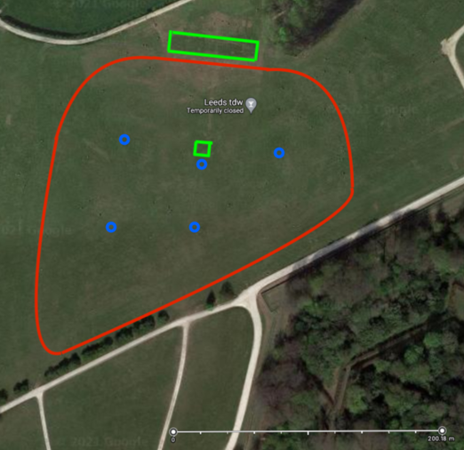
So we can now import this site map, scale it correctly, and start drawing features from it into the file.
The first thing we’ll want to do is a bit of housekeeping on the Layers side of things – make sure you’ve got the Layers window open, and click the plus button to add a layer for the site map, make sure it’s named something sensible, and then select the pen symbol on the right hand side of that line to enable editing on that layer. Now we can hide the Mesh layer using the eye symbol on it’s line.
Import the Map
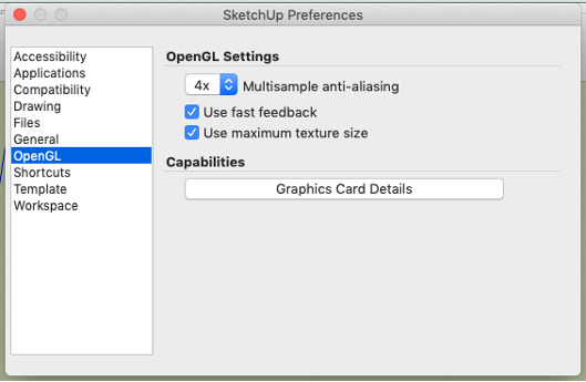
Next we want to go into SketchUp>Preferences>OpenGl and make sure the “Use maxiumum texture size” option is enabled – if you don’t do this it’ll massively compress the map on import to the point that it’s useless. The map still won’t be sharp, but it’ll be a lot better.
Next we can import the map using File>Import, click the first corner to the origin and then drag the second corner out until it’s roughly the right size (Tip: it’ll show you how big it is in the bottom right corner of the 3d View window)
Scale the Map
Then select the tape measure tool (T) and measure the scale bar on the map. In my case, the 200m bar measured at 184m, so we need to scale it up by a ratio of 200/184=1.0869. Tap (S) to get the scale tool, and then grab the yellow box on the top right corner and start dragging it out. Without clicking, type the ratio (1.0869 in this case) and hit enter. Use the tape measure to verify this on the scale bar again, and adjust if you need to.
Locate the Map
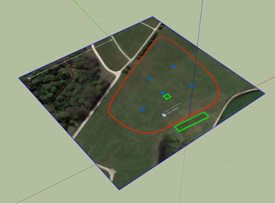
Now we can select the move tool (M), making sure that the map is selected, and select down stage centre on the map as our starting point. Moving this to the origin it should lock to the middle when you’re hovering over it. Then we can use the rotate tool to spin the map to line up with the stage like the image below:
Next we want to drop the map directly down 10m so that the geometry that we’re about to draw doesn’t interfere with the Mesh (yet) – Sketchup really doesn’t like intersecting lines and can get really weird if you’re not careful. Hit (M) and select the map, then the up arrow to lock movement to the vertical axes, then start lowering it, type 10, and hit enter.
Drawing the Features
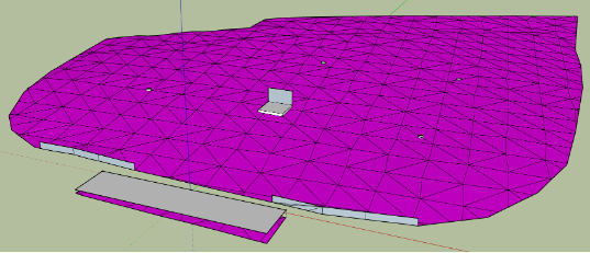
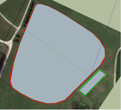
So now we can start drawing lines onto the top of the map - Create another layer for all the lines you’re about to draw and make sure you’re set to edit that layer then select the line tool (L) and start tracing around the outside of the audience area. Once you get back to where you started it should turn into a surface once you link back onto the first point. If ou do the stage as well you should have something like this:
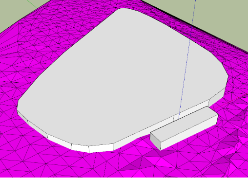
We can now use the pull tool (P) to pull this surface up through the mesh, I’d suggest just tapping 20m in on the keypad, but so long as it’s above the mesh it doesn’t matter. Turning the mesh visibility back on we should see something like this:
Now because up until now the mesh has been grouped, we need to right click on it and “explode” it, then select everything (Mesh and outline) and “right click>intersect faces>with selection” and it’ll cut the mesh along the outline that we’ve just pulled through.
With about 20 mins of back and forth you should be able to get most of the features onto the mesh and you’ll end up with something like this: